Data Normalization

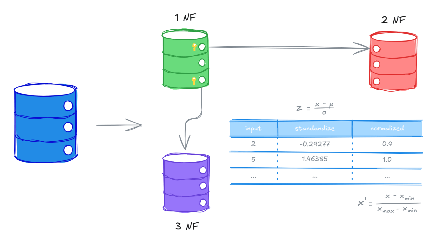
Big data can be challenging especially for organized and analyze due to its volume, variety, and complexity. To address this issue, normalization is commonly used.

However, normalization exists in 2 main forms: Database Normalization and Data Mining normalization.

Although they share similar goal of improving data usability, they are applied for different stages and purposes.

🗄️ Database normalization

Database normalization is used in database design to reduce redundancy and improve data integrity. It organizes data into multiple related tables involves dividing larger tables into smaller and ensures consistency.

Why Normalize?

• Eliminates duplicate data
• Reduces update, insert, and delete anomalies
• Improves data consistency
• Makes the database easier to maintain

There is a lot of stage form in database normalization that is 1NF, 2NF, 3NF and higher normal form typically used only in specialized databased design like BCNF, 4NF, 5NF.

Example (unnormalized table)

Original table

order_id	customer_name	products	quantities	prices	shipping_address
101	Alice	Phone, Charger	1, 2	500, 20	Jakarta, Indonesia
102	Bob	Laptop	1	1000	Bandung, Indonesia

Problems:

• Multiple products in one column
• Quantities & prices not atomic
• Hard to search/filter products

1NF

Rule:

• Each column must contain atomic (single) values.
• No repeating groups or arrays.

Convert table

order_id	customer_name	product	quantity	price	shipping_address
101	Alice	Phone	1	500	Jakarta, Indonesia
101	Alice	Charger	2	20	Jakarta, Indonesia
102	Bob	Laptop	1	1000	Bandung, Indonesia

2NF

Rule:

• Must be already in 1NF.
• No partially dependency on a composite key.

Assume composite key: (order_id, product) in 1NF table.

Dependencies:

• order_id → customer_name
• order_id → shipping_address

Decompose table:

orders

order_id	customer_name	shipping_address
101	Alice	Jakarta, Indonesia
102	Bob	Bandung, Indonesia

order_items

order_id	product	quantity	price
101	Phone	1	500
101	Charger	2	20
102	Laptop	1	1000

3NF

Rule:

• Must be in 2NF.
• No transitive dependency.

Observe: customer_name → shipping_address in 2NF orders table.

Problem: A customer’s address is determined by customer, not directly by the order.

Decompose table:

customers

customer_id	customer_name	shipping_address
C1	Alice	Jakarta, Indonesia
C2	Bob	Bandung, Indonesia

orders

order_id	customer_id
101	C1
102	C2

order_items

order_id	product	quantity	price
101	Phone	1	500
101	Charger	2	20
102	Laptop	1	1000

Boyce-Codd Normal Form (BCNF)

Rule:

• Must be in 3NF.
• For every functional dependency X → Y, X must be super key (candidate key).

Observed: dependency product → price in 3NF order_items table.

Problem: A product’s price is determined by the product itself, not by the order. So a non-key attribute (product) is determining another attribute (price).

BCNF issue: product → price because product is not a super key in order_items therefore, a non-key attribute is determining another attriubute.

Decompose table:

customers

customer_id	customer_name	shipping_address
C1	Alice	Jakarta, Indonesia
C2	Bob	Bandung, Indonesia

orders

order_id	customer_id
101	C1
102	C2

products

product	price
Phone	500
Charger	20
Laptop	1000

order_items

order_id	product	quantity
101	Phone	1
101	Charger	2
102	Laptop	1

4NF

Rule:

• Must be in 3NF/BCNF.
• No non-trivial multivalued dependencies (MVDs).

Because previous table already normalized so in this example we change the orders table in 3NF/BCNF like below to make example bad design for 4NF.

order_id	customer_id	product	coupon
101	C1	Phone	DISC10
102	C2	Phone	NEWUSER

Observe:

• order_id →→ product
• order_id →→ coupon

Problem: the table wourld force a cross-product combination like below and leads to redudancy and write (insert, update, delete) anomalies.

order_id	product	coupon
101	Phone	DISC10
101	Phone	NEWUSER
101	Laptop	DISC10
101	Laptop	NEWUSER

Decompose table:

orders (bcnf + 4NF base table)

order_id	customer_id
101	C1
102	C2

order_products

order_id	product
101	Phone
102	Phone

order_coupons

order_id	coupon
101	DISC10
102	NEWUSER

5NF / Join Normal Form (JNF)

Rule:

• Must be in 4NF.
• Can’t be decomposed further without losing information, except by joining on candidate keys.

5NF or Join is rare in real systems case in this example we gonna use real world scenario Suppliers - Parts - Projects 4NF tables.

supplies

supplier	part	project
S1	P1	J1
S1	P2	J1
S1	P1	J2
S1	P2	J2

Observe independent relationship:

1. supplier → part.
2. supplier → project.
3. part ↔ project compatibility (independent rule).

Problem: supplies table is incorrectly enforcing a ternary combination, which leads to redudancy and write (insert, update, delete) anomalies.

Decompose table:

supplier_parts

supplier	part
S1	P1
S1	P2

supplier_projects

supplier	project
S1	J1
S1	J2

part_projects

part	project
P1	J1
P2	J1
P1	J2
P2	J2

📊 Data mining normalization

Data mining normalization is used in data preprocessing for machine learning. It scales numerical values into a standard range so that features contribute equally to the model.

When normalization is important

It is especially important for:

• k-Nearest Neighbors (KNN)
• k-Means clustering
• Neural networks
• Principal Component Analysis (PCA)
• Support Vector Machines (SVM)

But less critical for algorithm:

• Decision trees
• Random forests

Common method:

Min-max normalization

Transform values into a specified range.

• Range usually [0, 1]
• Outliers sensitivity high

$$ x' = \frac{x - x_{\min}}{x_{\max} - x_{\min}} $$

Example:

If values range from 10 to 50 and $x = 30:$

$$ x' = \frac{30 - 10}{50 - 10} = 0.5 $$

Z-score normalization (standardization)

Transform data to have a mean of 0 and a standard deviation of 1.

• No fixed range
• Outliers sensitivity moderate

$$ z = \frac{x-\mu}{\sigma} $$

Where:

• $\mu$ = mean
• $\sigma$ = standard deviation

Example:

If $x = 70$, mean $ = 50$, standard deviation $ = 10$:

$$ z = \frac{70 - 50}{10} = 2 $$

Advantages:

• Less affected by outliers than Min-max normalization.
• Commonly used in statistical analysis.

Decimal scaling normalization

Moves the decimal point based on the maximum absolute value.

• Range typically (-1, 1)
• Outliers sensitivity moderate

$$ x' = \frac{x}{10^j} $$

Where $j$ is the smallest integer such that all normalized values fall between -1 and 1.

Example:

Suppose we have $x = [12, 345, -67, 8]$

Where:

• Maximum absolute value = 345
• It has 3 digits → so $j = 3$

Original ($x’$)	Calculation	Normalized
12	$\frac{12}{10^3}$	0.012
345	$\frac{345}{10^3}$	0.345
-67	$\frac{-67}{10^3}$	-0.67
8	$\frac{8}{10^3}$	0.008

Robust scaling (Median and IQR)

Use median and interquartial range (IQR), which are much less sensitive to extreme values.

• No fixed range
• Outliers sensitivity low

\[x' = \frac{x - \mathrm{median}(x)}{\mathrm{IQR}(x)}\]

Where:

• median(x) = middle value of the data
• $IQR(x) = Q3 - Q1$ (75th percentile minus 25th percentile)

Example:

Suppose we have dataset: [10, 12, 14, 16, 18, 20, 100]

Notice: 100 is an outlier

Where:

• median = 16
• Lower half = [10, 12, 14] → $Q1 = 12$
• Upper half = [18, 20, 100] → $Q3 = 20$
• $IQR = Q3 - Q1 = 20 - 12 = 8$

Original ($x’$)	Calculation	Scaled
10	$\frac{10-16}{8}$	-0.75
12	$\frac{12-16}{8}$	-0.50
14	$\frac{14-16}{8}$	-0.25
16	$\frac{16-16}{8}$	0
18	$\frac{18-16}{8}$	0.25
20	$\frac{20-16}{8}$	0.50
100	$\frac{100-16}{8}$	10.5

💡 Common idea

Both types of normalization aim to make data better organized, more useful, improve quality and effienciency but they solve different problems:

• Database normalization → makes data storage cleaner and more reliable.
• Data mining normalization → makes data values easier for algorithms to process.

How they connect in a real project

For example in a real system such as an e-commerce platform, both types of normalization are used at different stages of the data pipeline:

1. Data storage (Database Normalization)

   Store data customers, orders, and products in separate well structured tables. This ensure consistency and avoids duplication in the database.

2. Data extraction for analysis

   Data retrieved from databased for analytics or machine learning tasks.

3. Data processing (Data Mining Normalization)

   Features such as purchase amounts, customer age, and order frequency are normalized This ensured all featured on similar scale before training a machine learning model.

4. Model training

   A machine learning model is trained using the processed data for tasks like recommendation or prediction.